SPSS x Data Analysis
by Kumamon + Uncle G
All Regressions
ทำสำหรับ Model ที�่เป็นแบบ Regressions
ทดสอบ Normality
ค่าต้องกระจายแบบ Normal Distribution ไม่เบ้ไปมา
สร้าง P-Plots
- Analyze → Descriptive Statistics → P-Plots … → ใส่ตัวแปร → กด OK
สร้าง report statistics
- Analyze → Descriptive Statistics → Frequencies → ใส่ตัวแปร → ไปที่ Statistic แล้วติ๊กทุกอย่าง
- ยกเว้น Cut point, Percentile, Values are group midpoint → กด OK
สร้างกราฟ Historgram
- Analyze → Descriptive Statistics → Frequencies → Chart → Histogram + เลือก Show normal curve
ทำ K-S Test
- Analyze → Descriptive Statistics → Explore → ใส่ตัวแปรใน Dependent List → กด Plots → ติ้ก Normality plot with test → กด Continue → ไปที่ Option → เลือก Exclude cases pairwise
ทำ Levene's test
- Analyze → Descriptive Statistics → Explore → ใส่ตัวแปรใน Dependent List → กด Plots → ติ้ก Normality plot with test → ช่อง Spread vs Level with Lavene Test เลือก Untransformed
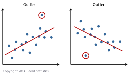
ลด Bias
เขียนแล้ว ด้านบน +SPSS x Data Analysis: Outlier-Detection
Heterogeneity of variance
Analyze → Descriptive Statistics → Explore → ใส่ Dependent List, Factor List → Plot → เลือก Untransformed
ถ้า significant (< 0.05) = ไม่มี Heterogeneity of variance = ดี
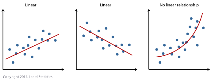
Linearity
ข้อมูลมีการเรียงอย่างเป็นเส้นตรง + เช็คว่าตัวแปรนั้นเป็นแบบ Continuous Graph → Chart Builder → Scatter/Dot → Simple Scatter → เอาตัวแปรไปใส่กราฟ → กด OK
Correlations Model
Analyze > Correlation > Bivariate → ใส่ตัวแปรเข้า Variable → ติ้กสื่งที่อยากได้
| Pearson’s Correlations | Spearman’s Correlations |
|---|---|
| สำหรับ Linear Relationship | สำหรับ Monotonic (Logsitics) Relationship |
| ค่าตัวแปรเป็นแบบ Continuous | ค่าตัวแปรเป็นแบบ Ordinal / Nominal |
ถ้า Spearman > Pearson → model มีความเป็น monotonic แต่ไม่ใช่ linear
ทำให้ถ้าอยากใช้ linear model → ต้องทำ Transformation ก่อน
Correlations Type
| Bivariate | Partial |
|---|---|
| ความสัมพันธ์ระหว่าง A กับ B | ความเกี่ยวข้องกัน โดยที่ไม่มี C มาเกี่ยวด้วย |
| ให้ทำการใส่ตัวแปรที่ช่อง Controlling For เพื่อทำให้ตัวแปรนั้นไม่เกี่ยวข้องกับตัวแปรที่คำนวณ |
- The bivariate correlation refers to the analysis to two variables, often denoted as X and Y – mainly for the purpose of determining the empirical relationship they have.
- The partial correlation measures the degree between two random variables, with the effect of a set of controlling random variables removed.
Chi-Square Test
การทดสอบ เพื่อวัดความเป็น Independent ของ 2 กลุ่ม
Assum**p**tion**s**
- ตัวแปรต้น → ระดับหมวดหมู่
- ข้อมูลที่เก็บมาอยู่ในหลายหมวดหมู่ไม่ได้ ต้องอยู่ในหมวดหมู่ใดหมวดหมู่หนึ่ง
Hypothesis
| Null | A & B มีความเป็น Independent ต่อกัน |
|---|---|
| Alternative | A & B ไม่มีความเป็น Independent ต่อกัน (Dependent ต่อกัน) |
How to use Analyze > Descriptive Statistics > Crosstabs → Statistic → เอาประเภทไปใส่ Column และ Row → เลือก Chi-Square, Norminal (Contingency Coefficient, Phi & Cramer’s V, Lambda)
ไปที่ Cell แล้วเลือก Count (Observed, Expected), Z-Test (ทุกอัน), Percentage (ทุกอัน), Residual (Standardized)
Fisher Exact Test หากว่าค่า Sample Size นั้นน้อย (ค่า Expected Count ในตารางคาดเดา) ให้ใช้ Fisher Exact Test แทน ไปที่ Exact → เลือก Exact
Interpretation โดยใช้ค่า Phi ( Φ ) หรือ/และ ค่า Cramér’s V
| Phi ( Φ ) | Cramér’s V ( φc ) | |
|---|---|---|
| Dimension Limitation | หากตารางไม่ได้เป็นแบบ 2x2 ห้ามใช้ | |
| ต้องมี 2 Dichtomous Variable | Nominal Variable |
แต่ถ้าตารางเป็น 2x2 จะใช้อันไหนก็ได้ ค่าเท่ากัน เพื่อแสดงความสัมพันธ์ ว่าแน่นแฟ้นขนาดไหน โดยดูค่า absolute ของมัน
ดูความ Significant ในช่อง Asymp. Sig ในตาราง Chi-Square Test sig ที่ >= 0.05 หากมีค่าที่ไม่ sig = มีค่าในตัวแปรใดตัวแปรหนึ่งแจกแจงผิดปกติ = มีความสัมพันธ์ระหว่างตัวแปร = Fail Null Hypothesis
Predictor (Independent Variable) Entry type
การเลือกนั้น ทำให้แล้วแต่ว่าแต่ละตัวแปรนั้นสำคัญมั้ย ถ้าไม่สำคัญก็ไม่ต้องเพื่ม
Forced Entry (ENTER Mode) [default]
- เข้าทีเดียวทุกตัว ไม่สนใจว่าตัวแปรไหนจะสำคัญหรือไม่ และไม่เอาออกด้วย
Enter and Remove (STEPWISE Mode)
- เลือกตัวที่สำคัญที่สุดก่อน แล้วค่อยๆเพื่มทีละตัว ตามความสำคัญ หากไม่สำคัญก็ไม่ต้องเข้า
โดยการเลือกนั้น SPSS จะเลือกจากค่า Chi-Square ที่เปลี่ยนไป ว่าไปในทิศทางที่ดีขึ้นหรือไม่
Durbin-Watson Statistics
ใช้เพื่อวัด Independent of Error (Observations)
How to use Linear Regression → ปุ่ม Statistics
Interpretation ค่าต้องอยู่เท่ากับ 2 ± 0.5 จะถือว่าดีมาก หากค่าเกิน 2 ± 2 จะถือว่ารับไม่ได้ มีปัญหา Independent of Error
โดยค่าที่น้อยกว่า 2 คือความสัมพันธ์เชิงลบ และมากกว่า 2 คือความสัมพันธ์เชิงบวก
Time Series / Autoregressive Analysis
เป็นการวัดว่าตัวแปร กับ เวลา นั้น มีความสัมพันธ์กันหรือไม่ และนำไป predict ค่าตัวแปรใหม่ โดยให้เวลามาหรือไม่
Autoregressive = เหมือน time series แต่มีหลายตัวแปรกว่า Time Series
Component of Time Series
| Trend | เกิด Trend กับเวลาหรือไม่ |
|---|---|
| Seasonality | ฤดูกาลเป็นสาเหตุของผลกระทบหรือไม่ |
| Cycle | เหมือน Season แต่อาจจะมี�ขนาดไม่เท่าๆกันได้ |
| Irregular Variation / Fluctuations | มีการเปลี่ยนแปลงแบบกระทันหัน เช่นอยู่ดีๆ sales ก็ peak ไปวันเดียว แล้วก็กลับมาเหมือนเดิม |
Tests
- ดูข้อมูลเราเป็นประมาณไหน
Analyze → Forecasting → Sequence Charts → ลาก ตัวแปรที่รวมทุกอย่างที่อยากดูไว้ใน variable → ตัวแบ่งช่วงเวลาไว้ใน Time Axis Label
- สร้างโมเดล
- ไปที่ Analyze > Forecasting > Create Traditional Model → นำตัวแปรที่เป็นแบบแยกไปใส่ใน Dependent Variable
- Method ตั้งเป็น Expert Modeler → กด Criteria → เอาตัวติ้ก “Expert modeler considers seasonal model” ออก → กด Continue (แล้วแต่ตัวแปรด้วย)
- tab Option
- เลือก “First Case after end of estimation period through a specific date” → ใส่ค่าเพื่อทำนาย
- tab Statistics
- เลือก Display fit measures , Stationary R Square, Goodness of fit และ Display forecasts
- tab Save
- เลือก Predicted Values ใน column save
- tab Plots
- เลือก Maximum absolute percentage error, Mean absolute percentage error, Series, Observed Values, Forecast
Reporting the result
SPSS จะออกค่าที่เราต้องการหา (ตอนที่ใส่ input เวลา) ออกมาให้ ว่ามันเดาอะไรออกมา
แล้วก็แค่นั้น เพราะสอนแค่นั้นจริงๆ
Vocabulary Time
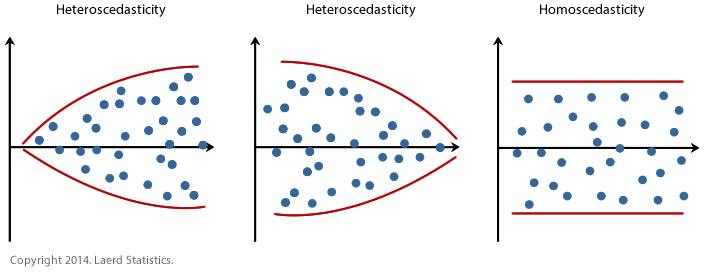
Heteroscedastic = Heterogeneity of variance = have different variabilities from others. Here "variability" could be quantified by the variance or any other measure of statistical dispersion.